Orbits, Energy, and Graphs
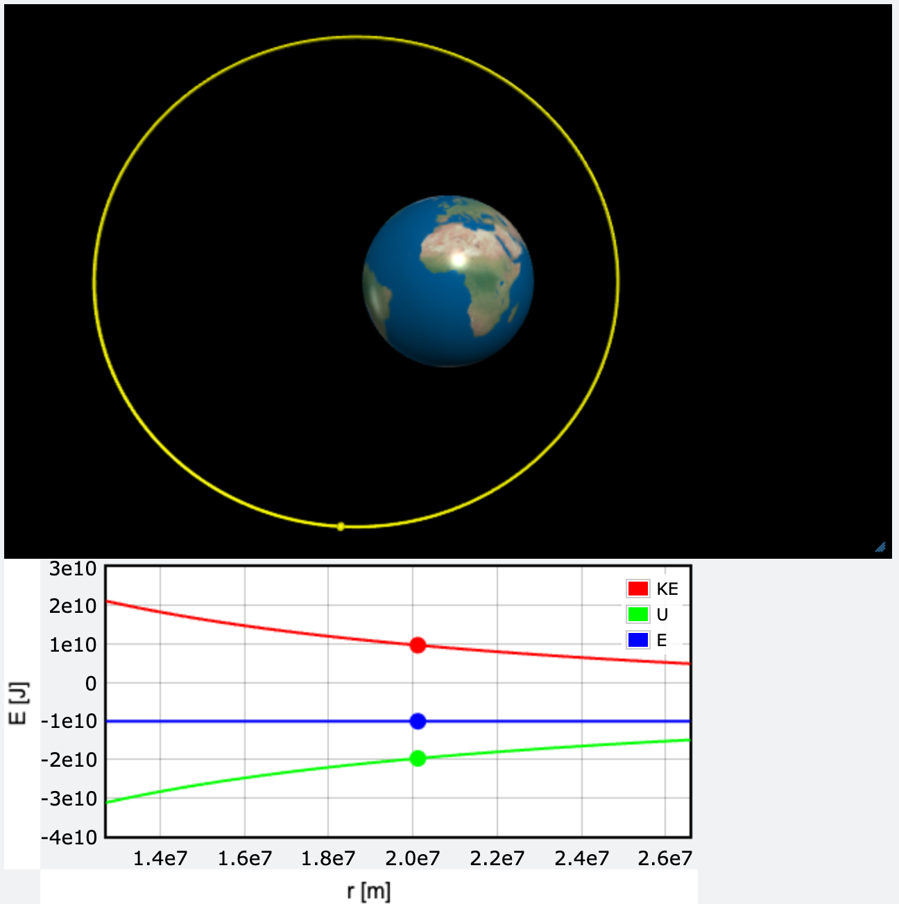
Click the image above!
As sophomore-year finals are wrapping up, I can finally continue this exciting endeavor in physics and space-related scientific programming.
Since my previous project was coded in VPython, I didn’t want to get too far ahead of myself, so I chose to build on that earlier simulation. While it is still based on the same theoretical formula—Newton’s Law of Universal Gravitation—I wanted to simplify the model. I knew it was getting serious when I brought out “textures.earth”—finally, some color.
Although this simulation is not as chaotic-looking as my N-body simulation, I decided to add an energy graph comparing kinetic energy, gravitational potential energy, and total energy throughout the spacecraft’s orbit. The graph shows how KE, U, and total E change in relation to the spacecraft’s distance from Earth’s center. This distance has to be calculated using the magnitude of the position vector, since the spacecraft’s radius from Earth is also a vector quantity.
When you run the simulation, especially after setting “dot=True” for each energy curve, the animation becomes pretty visually pleasing. As the spacecraft repeats its orbit, the x-axis value reverses because the spacecraft moves closer to and farther from Earth. As a result, the dots trace back and forth along the same three energy curves from one orbit to the next.
Overall, I enjoyed making more intuitive tweaks to my program that led to this simulation. It was a pretty fun way to build on my earlier project while also making the physics easier to visualize.
